



Quantifying and visualizing molecular dynamics can be a complex challenge for molecular modelers. Understanding where a molecular path spends the most time in specific coordinate spaces can provide invaluable insights, especially when making decisions in molecular design. This is where the 2D density map feature in SAMSON’s Path Analyzer proves incredibly useful.
Why use 2D density maps?
Imagine you are analyzing a molecule’s behavior along a path and you want to identify significant regions in the parameter space determined by two key observables—perhaps distance and RMSD, or energy versus radius of gyration. A 2D density map enables you to merge two saved scalar analyses and calculate a heatmap showing where the system spends the majority of its time. This allows you to identify preferred states or regions of interest in a reduced coordinate space.
For molecular modelers, this visualization is vital for summarizing complex dynamics. The heatmap highlights where the sampling density is highest, giving you a better understanding of trends and patterns in molecular motion or stability.
How to add a 2D density map in SAMSON
Setting up a 2D density map in SAMSON’s Path Analyzer is straightforward:
- Open Path Analyzer.
- Ensure you have at least two saved scalar analyses in the Analysis Tray. If not, create them by performing appropriate scalar analyses on your molecular path.
- Select the 2D density map option under Observable.
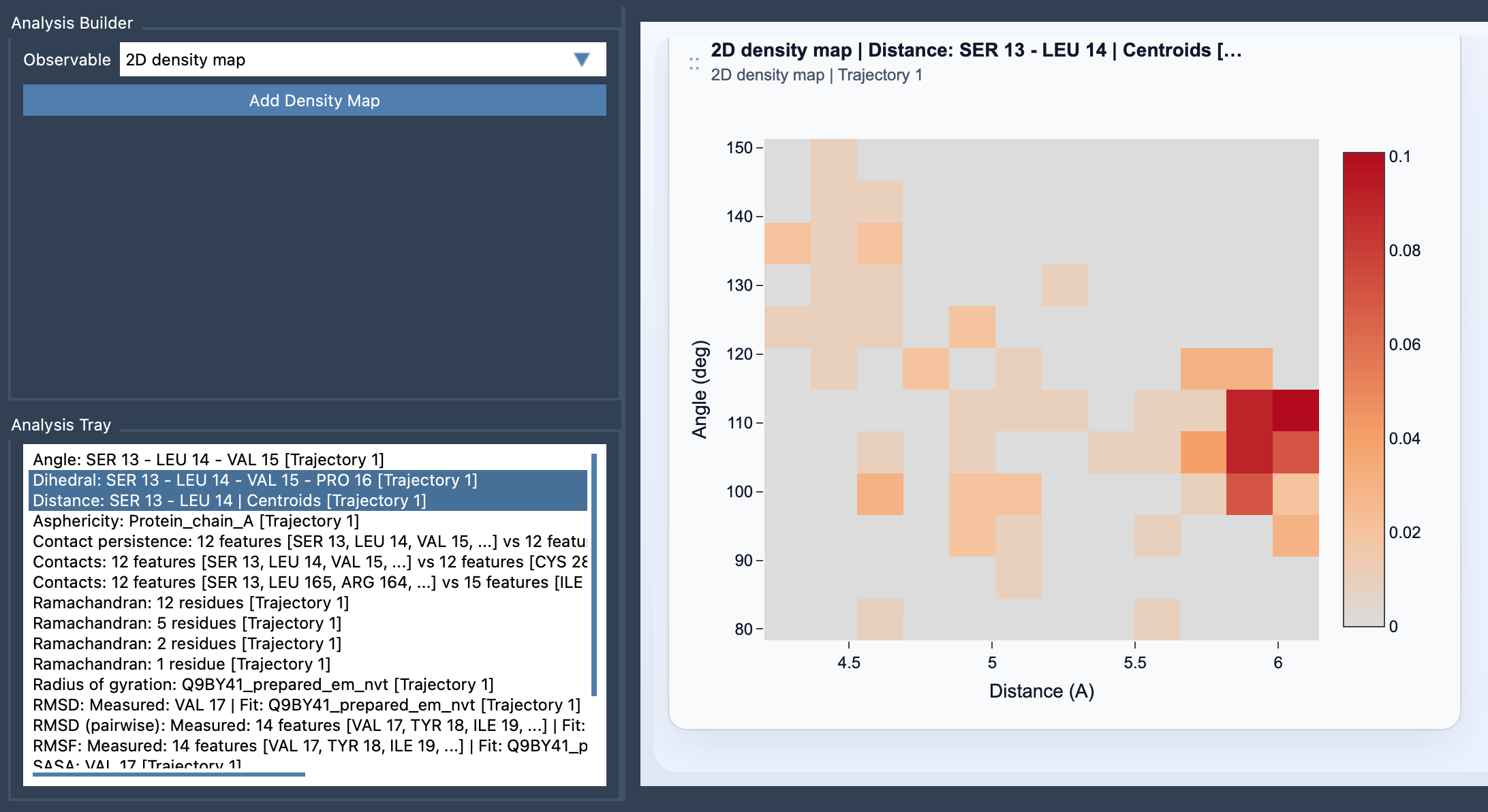
- Choose exactly two saved scalar analyses to combine into the map.
- Click Add Density Map.
Understanding the inputs
It’s worth noting that the 2D density map is a derived analysis, which relies on saved data in the Analysis Tray. The source analyses must be frame-wise computations performed on the same molecular path. This ensures consistency and relevance of the resulting heatmap.
What the 2D density map shows
The generated 2D density map is a heatmap displaying the density of points in your chosen two-observable space. For example, regions of higher density in the heatmap indicate where the molecule tends to spend more time. This makes it easier to focus on areas that potentially represent stable configurations or energetically favorable states.
Tips for effective use
- Select observables that represent orthogonal (independent) aspects of molecular motion. For instance, Distance vs RMSD to analyze physical movement, or Radius of gyration vs Energy to investigate molecular compactness and stability.
- Keep in mind that 2D density maps reflect sampling density, not energy. For energy-based visualizations, consider using the Energy Landscape tool in SAMSON.
Below is an example visualization of a 2D density map:
Learn more
Want to delve deeper? Explore the full documentation on 2D density maps at this link.
SAMSON and all SAMSON Extensions are free for non-commercial use. You can download SAMSON at samson-connect.net.