When Protein Endpoints Don’t Match: A Practical Route to a Transition Path

Two structures can show the states you care about and still refuse to fit into a straightforward transition-path workflow. A common reason is that the structures differ in residue count: the atoms in one endpoint do not map neatly onto the atoms in the other. Simply interpolating between them may therefore be impossible or misleading.

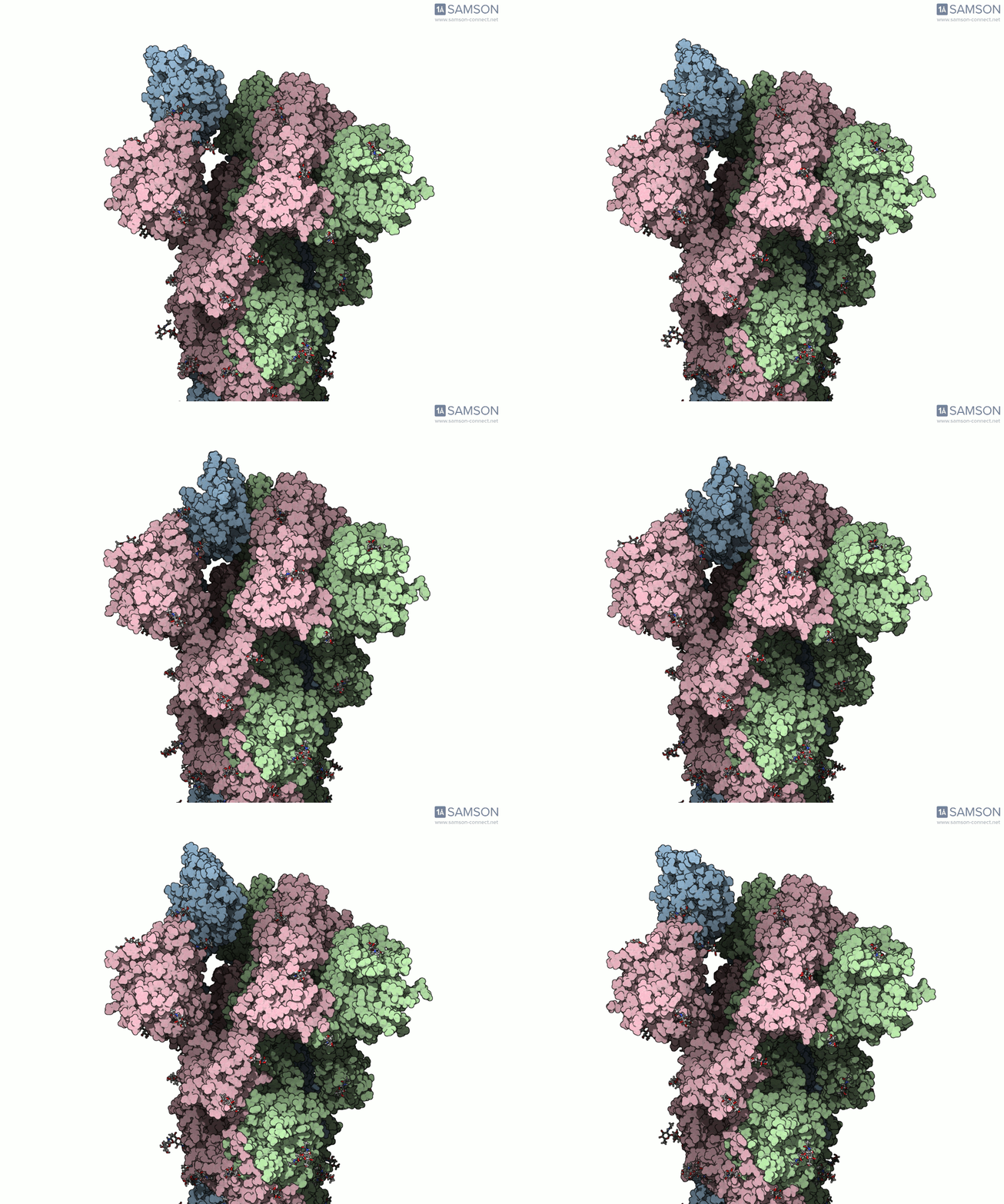
The SARS-CoV-2 spike opening example offers a useful case study in handling that mismatch. It uses the closed spike structure 6VXX and the open structure 6VYB to build an illustrative path. The workflow is not a general recipe for every protein, but it demonstrates an important modeling principle: prepare comparable endpoints before refining the path, and treat the result as a computational model rather than proof of the molecule’s exact motion.

Why matching endpoints matters

A transition-path method needs structures it can compare. In this example, the open and closed spike structures have different numbers of residues. That mismatch complicates the calculation because a path generated for one structure does not automatically provide a directly corresponding structure for the other.

The example also includes sugars attached to the spike. Before adding hydrogens, the workflow adjusts sugar bond orders using a Python script and SAMSON’s Python scripting module. Hydrogens are then added to both structures, followed by minimization steps. These preparation steps matter: they make the starting structures more suitable for the calculations that follow, rather than asking the path-generation method to compensate for avoidable input problems.

A two-stage way to address the mismatch

1. Generate an initial interpolation. The ARAP Interpolation Path module is used with the open structure, 6VYB, as the starting conformation and the closed structure, 6VXX, as the goal. The initial path corresponds to the starting structure.
2. Create a compatible closed endpoint. Because the structures differ in residue count, the workflow takes a closed-state conformation from the initial path, which has the open structure’s residue composition, and minimizes it. This provides a closed-like goal conformation that corresponds to the structure used for the path.
3. Recalculate the path. ARAP interpolation is run again using this newly obtained closed-state conformation as the goal. The point is not to hide the structural difference, but to construct endpoints that are compatible for the next calculation.
4. Refine the result. The P-NEB (Parallel Nudged Elastic Band) module is used to improve the path. In the documented example, this refinement took about 15 minutes on a laptop.

This sequence is useful to keep in mind whenever endpoint structures are not directly comparable: inspect what the path represents, create a compatible endpoint where appropriate, then refine. It also makes the workflow easier to troubleshoot, because preparation, interpolation, endpoint adjustment, and refinement are distinct stages.

What the trajectory can—and cannot—tell you

The resulting path helps visualize a possible structural transition from the closed, or down, state to the open, or up, state. In the open state, the spike’s receptor-binding region can recognize ACE2. The animations show the change from several views, while the downloadable files let you inspect the structures in more detail.

However, an interpolated and refined path should not be confused with an experimentally observed movie or a validated account of the timing and mechanism of a biological event. The trajectory files are provided as is and have not been experimentally verified. They may be useful for illustration or further calculations, but the documentation advises that they may require post-processing and additional validation before use.

The example is available as separate PDB trajectory files, a single PDB trajectory, or a SAMSON-format file. The SAMSON file includes the spike structure, open and closed conformations, and paths produced by ARAP and P-NEB. This makes it possible to inspect the workflow’s output rather than relying only on a rendered animation.

For modelers facing mismatched conformations, the key takeaway is practical: check structural correspondence before path generation, make preparation steps explicit, and keep the limits of the resulting trajectory visible to anyone who will use it.

Learn more in the original spike-opening tutorial, including the downloadable trajectory files and details of the SAMSON modules used.

Note: SAMSON and all SAMSON Extensions are free for non-commercial use. Get SAMSON.