



When two molecular groups appear close in a structure, it is tempting to treat one snapshot as the whole story. But a single distance may not tell you whether that arrangement is common, rare, or part of a broader pattern. A radial distribution function (RDF) helps answer a more useful question: across the selected path, how are the distances between two groups distributed?
This is especially helpful when examining local packing, solvation structure, or characteristic distances between a ligand and its surroundings. The curve can make recurring distance ranges easier to spot—but it also needs to be read with care. A peak is evidence of a population of distances, not by itself proof of a bond, a specific interaction, or its strength.
What the curve is counting
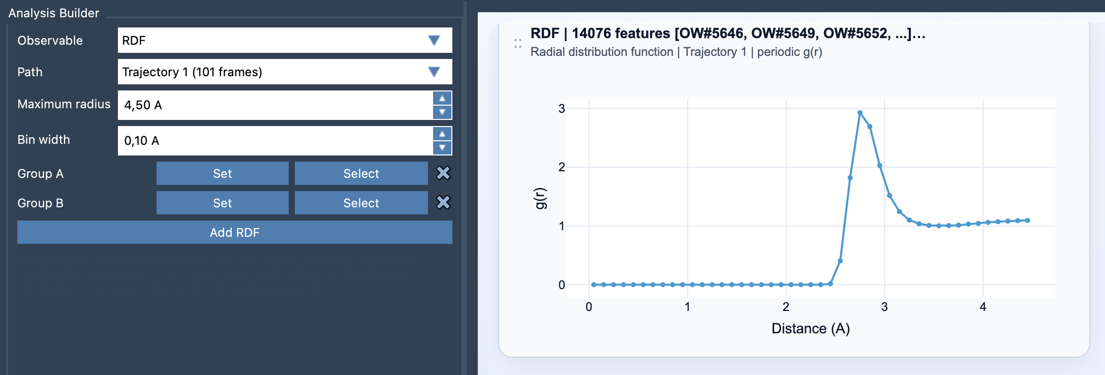
Path Analyzer builds the RDF from pairs of atoms in two selections, called Group A and Group B. It counts how many sampled pairs fall into distance shells around a radius r. The result is displayed as a one-dimensional curve against distance.
There is an important geometric detail: shells farther from the center have more volume than shells nearby. A shell’s approximate volume is 4πr²Δr, where Δr is the bin width. So a raw count at one distance range is not automatically comparable to a count at another. When valid periodic unit-cell information is available, Path Analyzer can normalize the counts against the expected ideal-gas occupancy and report a properly scaled g(r). Without the required periodic information, it instead shows an RDF-style curve in arbitrary units. In that case, read the curve as a relative distribution, not as an absolute, normalized RDF.
Set up a comparison that answers a real question
Start by choosing groups that reflect the question you want to investigate. For example, a solute–solvent selection can help you examine solvent organization around a solute; a ligand–pocket selection can summarize distances between the ligand and selected pocket atoms. Residue–residue subsets can be useful when you want to focus on particular parts of a larger structure. Both selections must contain atoms.
In Path Analyzer, choose RDF as the observable, select a path, define Group A and Group B, and set the maximum radius and bin width. Then select Add RDF. The maximum radius sets how far out the distribution is sampled. Choose it to cover the distance range relevant to your question; extending it farther is not automatically more informative.
Choose bin width for the pattern, not just the prettiest curve
Bin width controls radial resolution. Narrow bins can reveal finer detail, but they can also make the curve noisy. Wider bins smooth the appearance, while potentially merging nearby features. A practical approach is to begin with a moderate width, inspect the curve, and adjust it to see whether the features you care about remain interpretable. Avoid treating a tiny change in bin width as evidence that the underlying molecular behavior changed.
Interpret peaks with restraint
A peak indicates that sampled pairs occur more often around that distance range than in neighboring ranges, under the calculation’s normalization. Its position can suggest a characteristic separation worth investigating. But the RDF summarizes distances between the selected groups; it does not identify which atom pair caused a feature, explain its chemical origin, or establish that an interaction is favorable. Use chemically meaningful selections and interpret the curve alongside the molecular structure and other evidence.
Also remember that RDF cards are not frame-linked: they summarize the path globally rather than representing an individual frame. That makes them useful for an overall view, but not for locating a feature at a particular point in the path.
For the full setup details, see the Path Analyzer RDF documentation.
Note: SAMSON and all SAMSON Extensions are free for non-commercial use. Get SAMSON.