



A molecular trajectory can contain hundreds or thousands of frames. Watching the animation may show that two parts of a structure move, but it can be difficult to tell when an interface forms, whether it persists, or which residues are involved. Contact analysis helps turn that moving picture into two complementary summaries: a contact series over time and a contact map across the path.
Start with a question you can measure
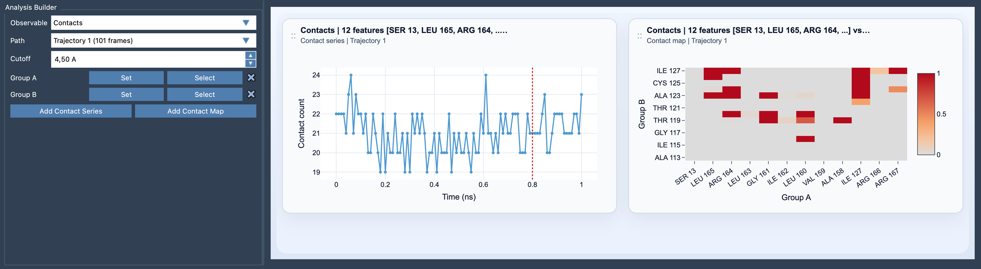
Before making a plot, decide which two parts of the structure you want to compare. They might be a protein and a ligand, two chains, or two domains. In Path Analyzer, choose Contacts as the observable, select a path, define Group A and Group B, and set a distance cutoff in ångströms (Å). Then add either a contact series or a contact map.
The choice of selection level matters. If you select broad clouds of atoms, a map can be difficult to interpret. Choosing residues, a ligand, chains, or domains as the root selections gives the map meaningful axes and makes it easier to connect a pattern to recognizable structural features.
Two views answer different questions
The contact series reports the total number of feature pairs in contact at each frame. It is useful for spotting changes in overall interface activity: a rise can coincide with an interface forming, while a fall can indicate that contacts are being lost. A changing curve is a cue to inspect the corresponding part of the path, not proof by itself of a particular biological event.
The contact map reports the occupancy of each feature pair over the full path. Occupancy is the fraction of frames in which that pair meets the cutoff. In practical terms, the map can help answer, “Which selected pairs account for the contacts I see?” A pair with high occupancy is within the chosen cutoff in many frames; a low-occupancy pair appears in fewer frames.
These summaries are most useful together. The series gives you a timeline of the total contact count, but it does not identify which pairs contribute to that count. The map identifies pairs and summarizes their occupancy, but its whole-path summary does not show exactly when each contact appeared or disappeared. Use the series to find periods of change, then use the map to identify the feature pairs worth examining.
Make the cutoff part of the interpretation
A contact is defined using the minimum inter-atomic distance between two features: the pair counts when that distance is below the cutoff you set. That makes the cutoff an important part of the result, not just a display setting. A different cutoff can change both the number of contacts and their occupancies, especially for pairs whose distances are near the threshold.
For a careful comparison, keep the selections and cutoff consistent across the paths or groups you are comparing. If a conclusion depends on a small change in the cutoff, treat it cautiously and check how the result responds to reasonable alternative settings. The analysis describes proximity under the chosen definition; contact counts alone do not establish binding strength, affinity, or the cause of a structural change.
A practical way to investigate a changing interface
- Select two biologically meaningful groups, such as a ligand and a protein region.
- Choose a path and set a cutoff in Å.
- Add a contact series to locate changes in the total number of contacts.
- Add a contact map to see which feature pairs contribute across the path.
- Return to the relevant frames and inspect the structural context of notable changes.
If you need the full binary time history of each contact pair, rather than an overall occupancy summary, use Contact persistence. For setup details and the equations behind both views, see the Contacts documentation.
Note: SAMSON and all SAMSON Extensions are free for non-commercial use. Get SAMSON.