



A molecular modeler often has two structures of the same protein and a practical question: how might the molecule move between them? The endpoint structures show where the protein starts and ends, but not the transition. Building a path is especially awkward when the structures do not contain the same number of residues, because their atoms may not correspond one-to-one.
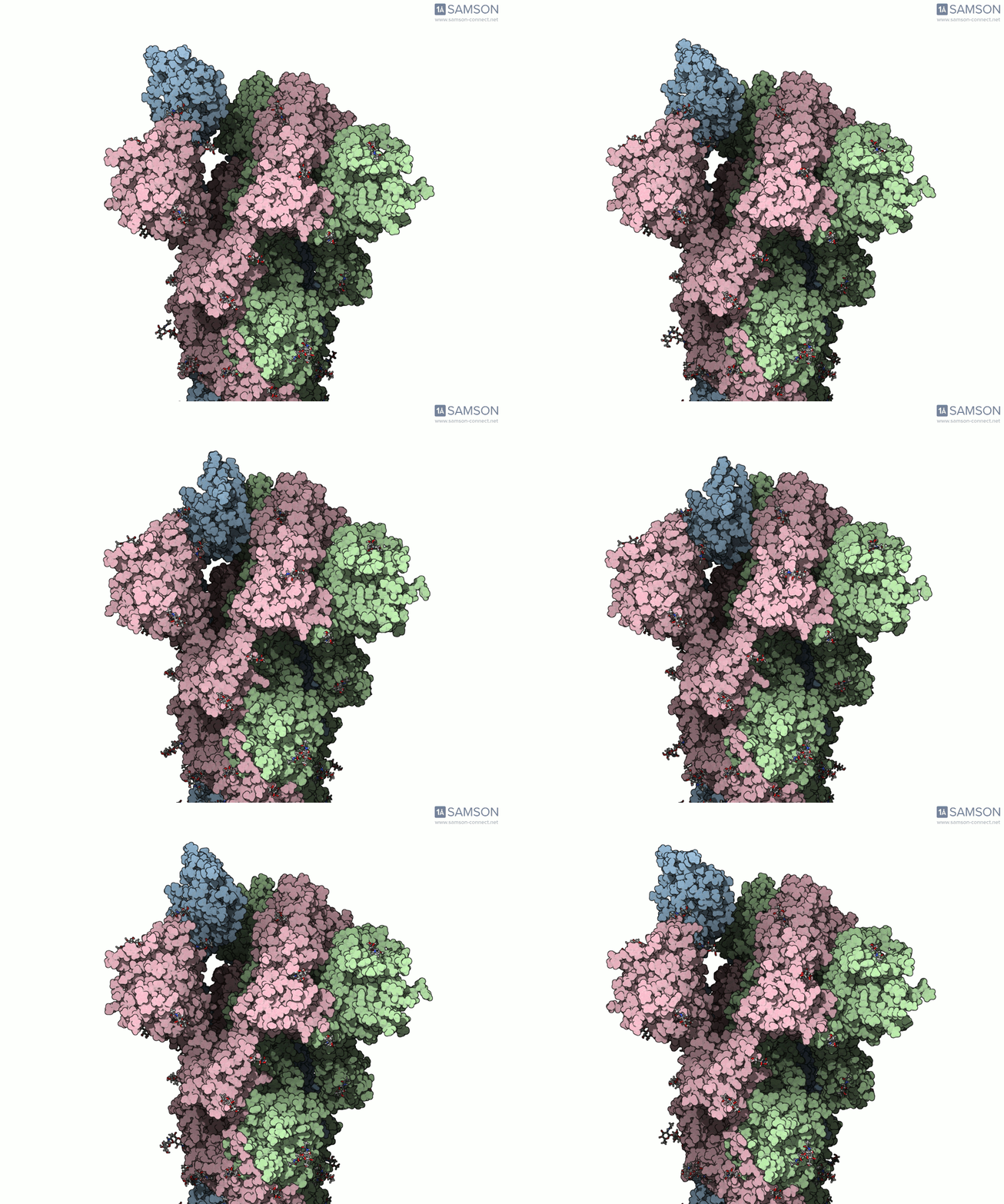
The SARS-CoV-2 spike provides a useful example. Its receptor-binding domain can adopt a closed, or “down,” state and an open, or “up,” state. The open state can recognize the human ACE2 receptor. The motion between these states is visually intuitive, but computing an illustrative path requires more than simply placing one structure beside the other.
Why endpoint structures are not enough
The example uses the closed spike structure PDB 6VXX and the open structure PDB 6VYB. These structures differ in the number of residues. That difference matters: a path-generation method needs a consistent set of atoms to move from one conformation toward another. If the endpoint representations do not match, the workflow must account for that before interpreting the resulting motion.
In SAMSON, the example first prepares both structures. Bond orders in the sugar molecules are adjusted with a Python script, then hydrogens are added and minimization steps are performed. These preparation steps are part of the example workflow; they are not evidence that every protein transition requires the same treatment.
A practical two-stage path workflow
The first stage uses the ARAP Interpolation Path module to generate an interpolated path between the structures. In the documented workflow, the open state is set as the starting conformation and the closed state as the goal. Because the path corresponds to the starting structure, the team then takes a closed-like conformation from that path and minimizes it. This gives them a closed-state-like endpoint represented with the open structure’s residue set.
They run the interpolation again, this time using that newly obtained conformation as the goal. The second stage applies the P-NEB (Parallel Nudged Elastic Band) module to improve the path. In the example, ARAP path generation took less than half a minute and P-NEB took about 15 minutes on a laptop. Those timings describe this particular example, not a general performance guarantee.

What to conclude—and what not to
A computed trajectory is a way to inspect a possible structural transition, not a direct recording of what happens in a virus. The example trajectories are provided “as is” and have not been experimentally verified. They may be useful for illustration or further calculations, but should be post-processed and validated before being relied on for scientific conclusions.
The downloadable files include individual PDB trajectory frames, a single PDB trajectory, and a SAMSON-format file. The SAMSON file includes the structure, open and closed conformations, and paths produced by ARAP and P-NEB; its conformations and animation can be explored in SAMSON. The accompanying motion views are useful for seeing the overall opening movement, while the structures and trajectory provide material for closer inspection.
The broader lesson for molecular modeling is to treat path construction as a workflow: prepare endpoints, address differences in their representation, generate an initial path, refine it, and keep the limits of the result visible. For the full walkthrough, files, and module details, learn more in the original documentation.
Note: SAMSON and all SAMSON Extensions are free for non-commercial use. Get SAMSON.