From Two Protein Structures to a Motion Path: Handling the Gap Between Endpoints

A molecular modeler often has two structures of the same protein and a deceptively simple question: what might the transition between them look like? The endpoints may be experimentally determined, but the route between them is not. A direct interpolation can be difficult to interpret—and even setting up a calculation can become complicated when the structures differ in residue count.

The SARS-CoV-2 spike provides a useful example of how to approach this problem. Its receptor-binding domain moves between a closed, or “down,” state and an open, or “up,” state. The open state can recognize the human ACE2 receptor. The animation below shows the computed opening and closing motion from the side.

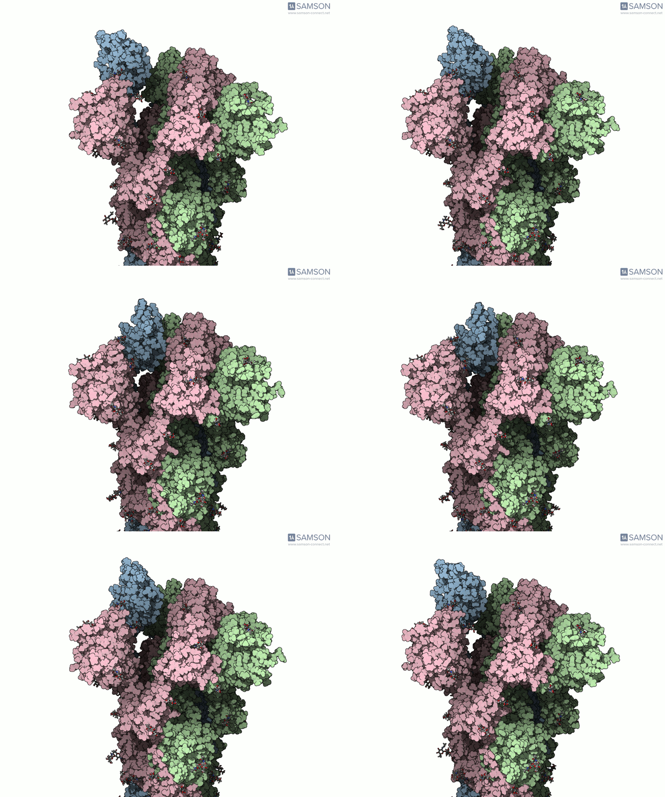
Why two endpoints are not always enough

The example begins with two known structures: closed-state PDB 6VXX and open-state PDB 6VYB. They differ in their number of residues, which means they cannot simply be treated as identical structures with matching atoms throughout. That mismatch affects how a path is constructed: the path must correspond to a consistent set of atoms, and the two endpoint conformations need to be made compatible for the calculation.

This is a broadly useful lesson for transition-path work. Before choosing an interpolation or optimization method, check whether the structures represent comparable molecular systems. Differences in residue coverage, missing regions, and preparation can matter as much as the choice of path algorithm.

A practical workflow for the example

1. Prepare both structures. Bond orders in the sugar molecules were adjusted with a Python script and SAMSON’s Python scripting module. This was needed before adding hydrogens; bond orders for residues are set on import.
2. Add hydrogens and minimize. Hydrogens were added to both structures, followed by minimization steps. This provides prepared starting and goal conformations for the path workflow.
3. Generate an initial path. The ARAP Interpolation Path module was used to interpolate between the open and closed conformations. The documented calculation took less than half a minute on a laptop. ARAP generates a path for the structure corresponding to its starting conformation.
4. Address the residue-count mismatch. Because the endpoint structures differ in residue count, a closed-state conformation was taken from the initial path, which corresponds to the open-state structure, and minimized. This created a compatible goal conformation for another ARAP path calculation.
5. Refine the path. The P-NEB (Parallel Nudged Elastic Band) module was then used to improve the path. This step took about 15 minutes on a laptop in the reported workflow.

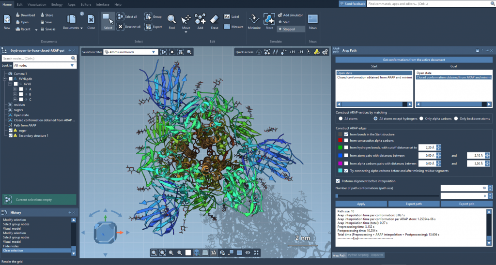
The sequence matters: interpolation supplies a route between structures, while the later P-NEB step refines that route. When endpoints are not directly compatible, the workflow may need an intermediate conformation that matches the atom set used for the path. That is not a detail to hide; it is part of making the calculation interpretable and reproducible.

Read the trajectory with the right caveat

The downloadable trajectory is an illustration of a possible spike motion, not an experimentally verified account of the exact route taken by the protein. The documentation notes that the files are provided “as is” and may require post-processing or further validation before being used in additional calculations. Keep that distinction clear: known structures define the endpoints, while a computed path is a model connecting them.

The SAMSON-format file includes the spike structure, open and closed conformations, and paths computed with ARAP and post-processed with P-NEB. The trajectory can be inspected in SAMSON, where the conformations and animation are available from the document view. Downloadable PDB trajectory files and a single PDB trajectory are also provided.

For molecular modelers, the practical takeaway is simple: inspect endpoint compatibility first, prepare the structures consistently, and treat a generated path as a hypothesis to examine—not as direct experimental evidence. The spike example makes those steps visible, including the extra work required when the structures do not have the same residue count.

Learn more in the original documentation, including the trajectory downloads, module details, and related tutorials.

Note: SAMSON and all SAMSON Extensions are free for non-commercial use. Get SAMSON.