



A molecular path can produce a lot of measurements: distances, energies, RMSD, radius of gyration, solvent-accessible surface area, and more. Looking at each value on its own may tell you how it changes, but not whether two observables change together. That gap can make it difficult to spot coordinated motion, distinguish groups of conformations, or identify which part of a path deserves a closer look.
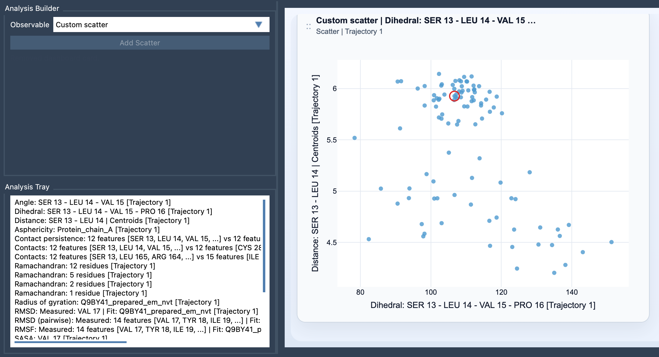
A custom scatter plot in SAMSON’s Path Analyzer provides a direct way to compare two saved scalar analyses. Each point represents one sampled pair of values. Instead of reviewing two separate analyses, you can inspect how their values are distributed together and ask a more focused question about the path.
Start with a question, not just two measurements
The most useful pairs are chosen to answer a scientific question. For example, you might ask whether a particular distance tends to increase as energy changes, whether RMSD varies alongside the radius of gyration, or whether solvent-accessible surface area changes with a distance of interest. These examples are not conclusions in themselves; they are ways to turn a broad set of measurements into a specific comparison.
Before creating the plot, decide what relationship would be meaningful for your system. If the points generally move in one direction across the plot, the two observables may vary together. If they tend to move in opposite directions, they may show an opposing pattern. Separate groups of points may suggest that the sampled path contains distinct regions in the chosen observable space. These visual patterns can guide investigation, but a scatter plot alone does not establish why a relationship occurs or prove that one observable causes another.
Build the comparison
- Open Path Analyzer.
- Create or reuse two saved scalar analyses in the Analysis Tray.
- Choose Custom scatter in Observable.
- Select exactly two saved scalar analyses in the tray.
- Click Add Scatter.
Custom scatter is a derived analysis: its inputs come from the Analysis Tray rather than from direct atom selections. Both source analyses must be scalar analyses. Thinking of the plot as a comparison between two existing measurements can help keep the workflow clear: first produce the observables you need, then compare them.
Use the path connection to investigate points
When both source analyses come from the same path and remain frame-linked, the scatter plot can stay connected to the current frame. In that situation, clicking a point can move the path to its corresponding frame. This makes the plot more than a summary: a point that looks unusual can become a starting place for inspecting the associated structure or path state in context.
A practical way to work is to first notice a pattern or outlier, then select a point and examine the corresponding frame when frame-linking is available. Compare neighboring regions of the path and consider whether the visual pattern fits the molecular question you started with. Keep in mind that the plot represents sampled pairs of scalar values, so interpretation depends on the analyses and path you supplied.
From overview to deeper analysis
A scatter plot is often a useful first look before moving to a more specialized view. If you want to examine how values are distributed across a two-dimensional space, the documentation also suggests a 2D density map. For an energy-focused view, see the Energy landscape. The scatter plot helps you begin with the relationship between two observables; those other views can help you explore the data from a different angle.
For the complete procedure and details, see the Custom Scatter documentation.
Note: SAMSON and all SAMSON Extensions are free for non-commercial use. Get SAMSON.