



A common challenge in molecular modeling is that two structures show where a protein starts and ends, but not how it might get from one state to the other. Simply switching between the structures hides the transition—and differences in residue counts can make building a continuous path more complicated. The SARS-CoV-2 spike opening example offers a useful case study in turning endpoint structures into an inspectable, computationally generated motion.
What the endpoints tell you
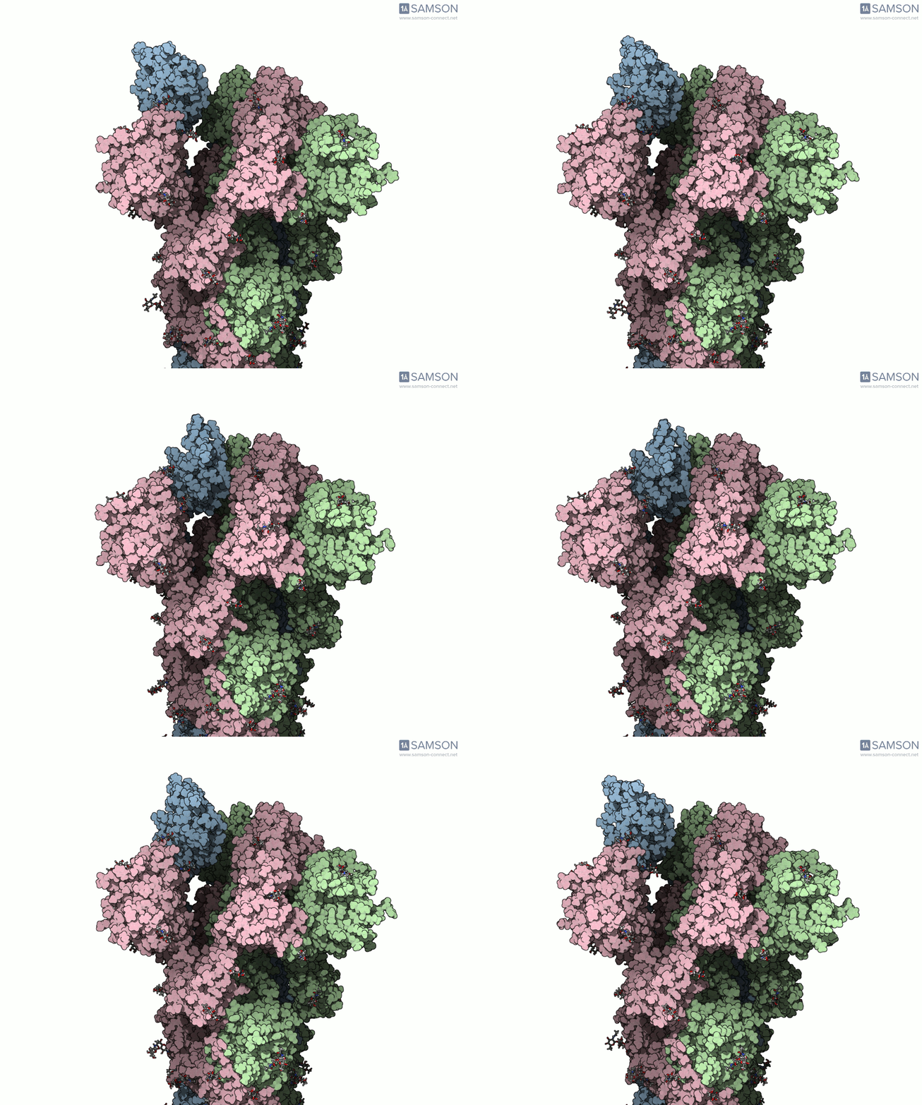
The example uses the closed spike structure PDB 6VXX and the open structure PDB 6VYB. In the open state, the receptor-binding region can engage ACE2, a protein found on the surface of some human cells. The spike is a three-part assembly, and the opening motion involves one of its receptor-binding regions moving upward.
These structures are informative endpoints, but they do not, by themselves, provide a continuous route between conformations. The structures also differ in the number of residues, which means a direct interpolation is not a straightforward one-to-one comparison. That mismatch is an important practical reminder: before computing a path, check whether the structures have compatible contents and decide how to handle differences.
A workflow that addresses the mismatch
The documented workflow prepares both structures before generating and refining a path:
- Prepare the input structures. Bond orders in sugars were adjusted with a Python script and the SAMSON Python scripting module. This was needed before adding hydrogens; bond orders for residues are set by SAMSON during import.
- Add hydrogens and minimize. Hydrogens were added to both structures, followed by minimization steps.
- Generate an initial path. The ARAP Interpolation Path module was used to interpolate between the known states. In the documented setup, the open state (6VYB) was the starting conformation and the closed state (6VXX) the goal. The initial path took less than half a minute on a laptop.
- Make the endpoint compatible with the path. Because the two endpoint structures have different residue counts, a closed-state conformation was taken from the path—which represents the starting structure—and minimized. This gave the next interpolation a closed-like target with the path’s structure.
- Refine the path. ARAP interpolation was run again using the newly obtained closed-state conformation as the goal. The resulting path was then improved with the Parallel Nudged Elastic Band (P-NEB) module, a step that took about 15 minutes on a laptop in this example.
The key lesson is not that every protein transition needs these exact steps. It is that path generation depends on thoughtful preparation: endpoint differences may need to be resolved, and an initial interpolated route can be refined rather than treated as the final answer.
Inspect the motion—and keep its limits in view
The example trajectory is available as separate PDB trajectory files, a single PDB trajectory, or a SAMSON-format file:
- Download the set of PDB trajectory files
- Download the single PDB trajectory
- Download the SAMSON-format file
The SAMSON file contains the spike structure, open and closed conformations, and paths from ARAP and P-NEB. The conformations can be restored by double-clicking them, and the path animation can be started or stopped by double-clicking the path. Viewing a trajectory can make structural changes easier to interpret than comparing two static images, but an animation should not be mistaken for experimental evidence. The published trajectories are provided “as is”; they have not been experimentally verified and may need further processing or validation before use in calculations.
For more context on the structures, visualizations, and complete workflow, read the original spike-opening tutorial.
Note: SAMSON and all SAMSON Extensions are free for non-commercial use. Get SAMSON.