



Molecular modelers frequently grapple with questions of spatial distribution: How are certain groups of atoms arranged relative to one another? Are there consistent patterns in their local packing or solvation structure? Understanding these patterns can be pivotal when analyzing molecular interactions, predicting properties, or optimizing designs. This is where the Radial Distribution Function (RDF) analysis in SAMSON’s Path Analyzer becomes a powerful tool.
What Does RDF Analysis Do?
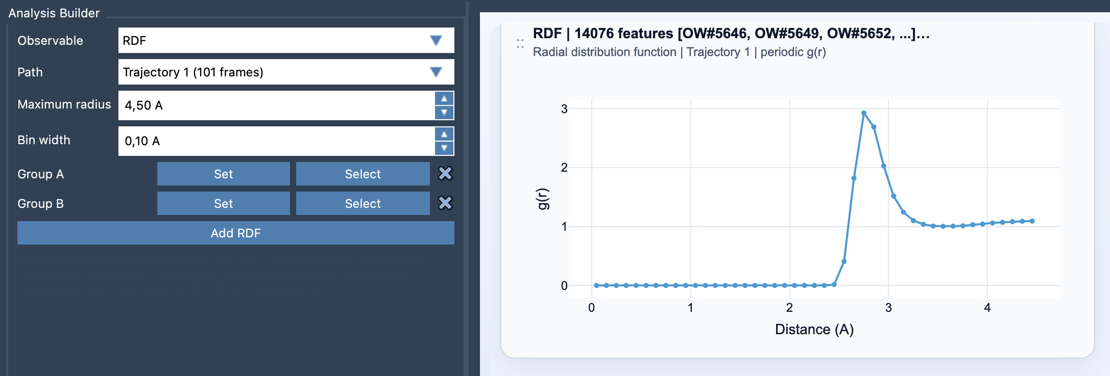
The RDF analysis in SAMSON computes the radial distribution function of atomic groups over a distance. Essentially, it helps quantify how atoms in one group (Group A) are distributed around another group (Group B). By visualizing this as a density versus distance curve, modelers can identify local packing, solvation shells, or characteristic interaction distances.
For example, in a protein-ligand system, the RDF might illuminate the key distances at which solvent molecules cluster around crucial residues—or how ligand atoms interact with a pocket.
Step-by-Step: Adding an RDF Plot
Generating an RDF plot in SAMSON is straightforward:
- Open the Path Analyzer.
- Select RDF as the observable property to compute.
- Define the Path.
- Assign Group A and Group B from your system. For meaningful results, use chemically relevant groups, such as solute-solvent pairs or specific residue subsets.
- Set the Maximum radius (the distance range for the calculation) and Bin width (the radial resolution).
- Click Add RDF.
This process results in a visual RDF curve, giving you immediate insights into the spatial relationships within your system.
Key Considerations
- Bin width: Choosing the right bin width is crucial. A very fine bin width might make the curve noisy, obscuring key features. Conversely, a very coarse bin width might oversimplify essential patterns. Experimentation with meaningful ranges is advised.
- Chemical context: The groups you analyze define the biological or chemical relevance of your curve. For example, analyzing solvent density around specific ligand atoms or the interaction distances between residues offers more actionable insights than random atom subsets.
- Normalization: If periodic boundary cell information is available, SAMSON can normalize the curve to account for ideal-gas occupancy within the shell, providing a scaled
g(r). If this information is unavailable, the calculated RDF will still offer insights, but in arbitrary units. - Global summary: RDF plots in SAMSON summarize data over the entire path for consistency, rather than being frame-specific.
What the Curve Tells You
Once you generate the RDF plot, the peaks on the curve correspond to distances at which group interactions are frequent. A significant peak, for instance, might reflect a solvation shell around a solute or highlight a critical ligand-pocket interaction distance. Such quantitative insights can guide structure-based optimizations.
Pro Tips for Better Analysis
- Use chemically meaningful groups for Groups A and B, such as solute-solvent pairs or ligand-target residues.
- Balance bin width to capture key features without introducing noise.
- If available, leverage the normalization feature to interpret your results in physically meaningful scales.
- Remember, RDF visualizations provide a global summary of paths, helping you study aggregate trends or characteristics.
RDF analysis is a treasure trove for molecular modelers looking to understand local interactions. Whether you’re exploring solvent spheres, ligand binding, or inter-group distances, SAMSON’s Path Analyzer lets you identify trends that could transform your molecular design workflow.
To explore more about RDF analysis and its settings in SAMSON, visit the official RDF documentation.
Note: SAMSON and all SAMSON Extensions are free for non-commercial use. You can download SAMSON at https://www.samson-connect.net.