



Molecular modelers often grapple with analyzing the spatial organization and interactive dynamics within complex molecular systems. Whether you’re studying solvation structures, local packing around specific groups, or characteristic interaction distances, the Radial Distribution Function (RDF) can be a crucial tool in your molecular modeling toolbox. Here, we’ll dive into the usage of RDF analysis, discuss common pain points it can solve, and highlight key inputs for its effective application.
What is RDF Analysis?
RDF analysis computes the radial distribution function between two predefined groups of atoms or molecules. It essentially measures how particle density varies as a function of distance from a reference particle. This is invaluable if you want to uncover patterns of local ordering or study solvation layers or ligand-pocket interactions.
In the simplest terms, RDF counts how many sampled pairs fall within a shell at a given distance. This can reveal peaks related to solvation shells or molecular packing, which would otherwise remain hidden in complex simulations.
How to Add an RDF Plot
Here’s a step-by-step guide to adding an RDF plot in SAMSON’s Path Analyzer:
- Open the Path Analyzer app.
- Select RDF under the Observable options.
- Choose the specific Path you want to analyze.
- Define the two groups of interest – Group A and Group B.
- Set parameters: Maximum radius for the sampling range and Bin width for the radial resolution.
- Click on Add RDF, and the plot will be generated.
Tips for Effective RDF Use
While the setup process is straightforward, ensuring meaningful results often requires thoughtful preparation and parameter selection:
- Use chemically meaningful groups for Group A and Group B. For example, solute-solvent interactions can highlight solvation shells, whereas ligand-pocket interactions can reveal binding properties.
- Choose a bin width that balances resolution and noise. A finer bin width can resolve smaller features in the RDF, but it might introduce noise, while too coarse a bin width may obscure critical details.
- If periodic simulation cell information is available, SAMSON can normalize the RDF data against ideal-gas occupancy, providing a properly scaled
g(r). This gives more meaningful insights into structured systems.
Key Inputs and Insights
For RDF analysis, two atom-containing selections are required. The Maximum radius parameter determines how far from the reference group the distribution is sampled, while the Bin width dictates the detail level of the curve. By fine-tuning these inputs, you can adjust how the RDF captures the structural characteristics of your system.
The result of RDF analysis is a one-dimensional curve, where the y-axis represents particle density, and the x-axis represents radial distance. Peaks in the curve correspond to regions of higher density – essential for identifying solvation shells, ligand interaction distances, and crystal packing characteristics.
Visualizing the Power of RDF in Action
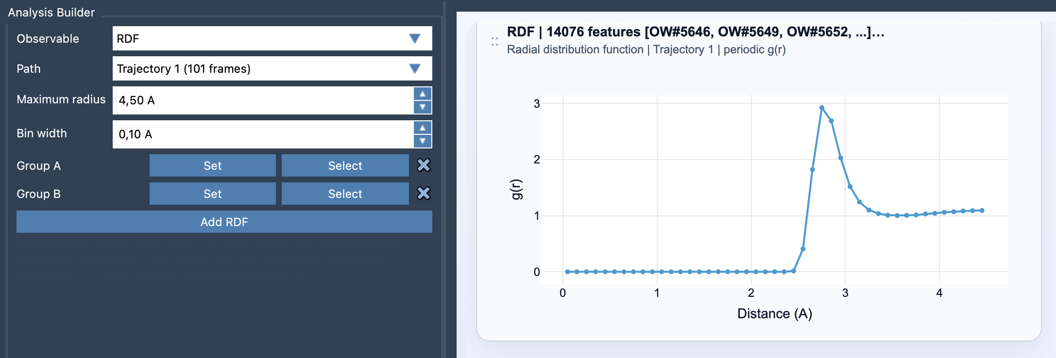
The generated RDF plot, such as the one shown above, allows molecular modelers to uncover patterns that might not otherwise be observable in complex molecular systems.
Conclusion
Understanding the radial distribution function through RDF analysis can greatly simplify tasks ranging from solvation analysis to studying molecular ordering. SAMSON’s Path Analyzer makes this process accessible through its user-friendly interface. With the ability to customize parameters such as bin width and maximum radius and integrate system-specific data, the tool ensures you derive meaningful insights from your molecular simulations.
To dive deeper into RDF analysis, visit the official documentation page here. Mastering this method can unlock a new depth in your molecular modeling studies.
SAMSON and all SAMSON Extensions are free for non-commercial use. Get started today by downloading SAMSON from here.