



For molecular modelers and computational chemists, understanding local packing, solvation structures, or the characteristic interaction distances between atoms or molecules can be critical. The Radial Distribution Function (RDF) is a powerful tool to achieve exactly that. But how do you actually compute and visualize RDFs effectively? If you’re a SAMSON user, the Path Analyzer module provides a streamlined way to create RDF plots with just a few steps. Read on to learn how this works, and how it can simplify your analysis.
What is the RDF Analysis?
The RDF analysis computes the radial distribution function between two groups of atoms or molecules. Essentially, it helps to determine the spatial distribution of atoms in relation to a reference point. This is invaluable when studying aspects like:
- Local packing densities.
- Solvent structure around a solute.
- Key interaction distances between molecules or within a molecular complex.
In practical applications, RDFs can reveal structural organization in simulations or experiments, making them essential in molecular dynamics, structure prediction, and materials science.
Step-by-step: Setting Up RDF Plots in Path Analyzer
Here’s how you can set up RDF plots using the Path Analyzer module in SAMSON:
- Open the Path Analyzer interface in SAMSON.
- Select RDF under the Observable settings.
- Specify the Path you’d like to analyze. This is the trajectory or structural path along which the RDF will be computed.
- Define your two atom-containing groups: Group A and Group B. These are the groups between which the radial distribution will be calculated—such as solute and solvent atoms, or backbone and side-chain groups of a protein.
- Set parameters for the analysis:
- Maximum radius: Defines the distance range to sample the radial distribution.
- Bin width: Controls the resolution of the radial bins (smaller bin widths give finer resolution but may introduce noise).
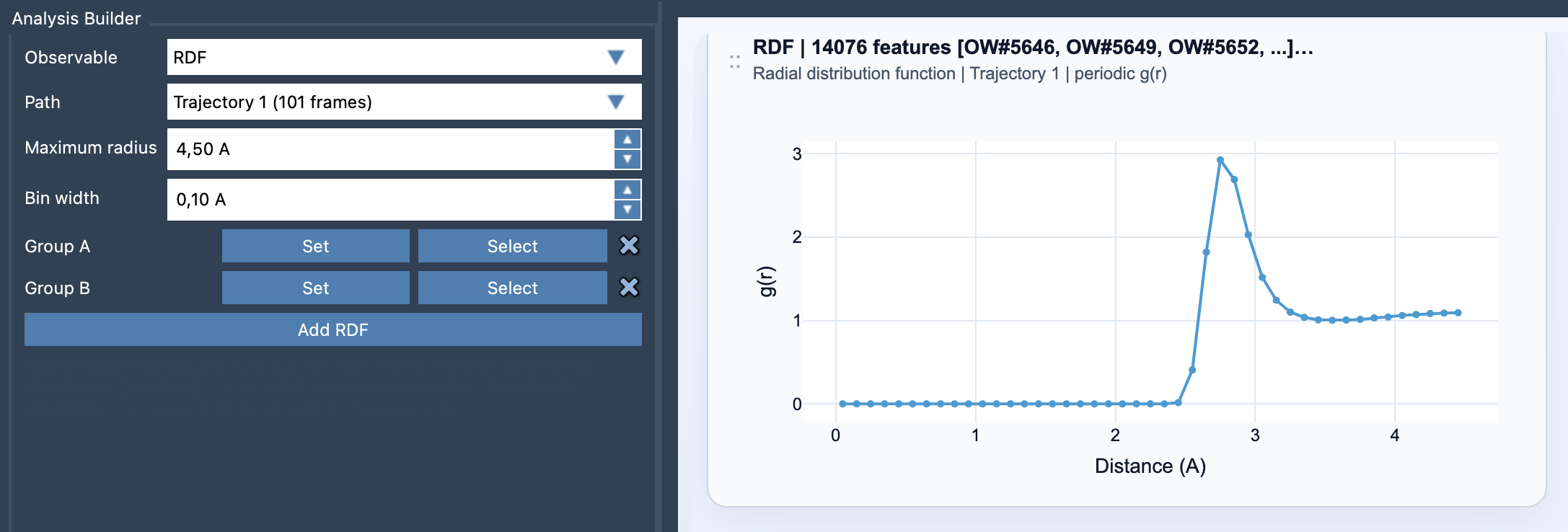
- Click on Add RDF to generate the plot. The resulting RDF card will display a smooth one-dimensional curve of density versus radial distance.
Tips for Meaningful Results
To make the most out of your RDF analysis, consider the following tips:
- Choose chemically meaningful groups for Group A and Group B. For example, ligand-pocket interactions, solute-solvent relationships, or residue-residue subsets in biomolecular systems offer actionable insights.
- Select a bin width that balances resolution and signal clarity; smaller bin widths can provide detailed information but might render a noisy curve if your dataset is sparse.
Exploring Normalization and Beyond
Path Analyzer can also normalize the RDF based on periodic cell information. When provided with valid unit-cell details, it computes an ideal-gas occupancy of the radial shell, producing a normalized g(r). This makes the curve more interpretable and allows for a rigorous comparison with experimental or theoretical models.
If periodic cell data is unavailable, Path Analyzer falls back on an RDF curve in arbitrary units for visualization purposes without normalization.
Note: RDF cards are not frame-linked because they summarize the trajectory globally, rather than frame-by-frame.
Quick Example Visualization
Below is an example RDF curve generated through Path Analyzer. This one-dimensional plot helps visualize the density of atoms over distance clearly:
Conclusion
By following the steps outlined above, you can easily compute and visualize RDF plots in SAMSON using the Path Analyzer module. This is an effective way to glean deeper insights into your molecular system’s structural characteristics. To fully explore the RDF capabilities or for further details, visit the official RDF documentation page.
Note: SAMSON and all SAMSON Extensions are free for non-commercial use. Get SAMSON at https://www.samson-connect.net.