



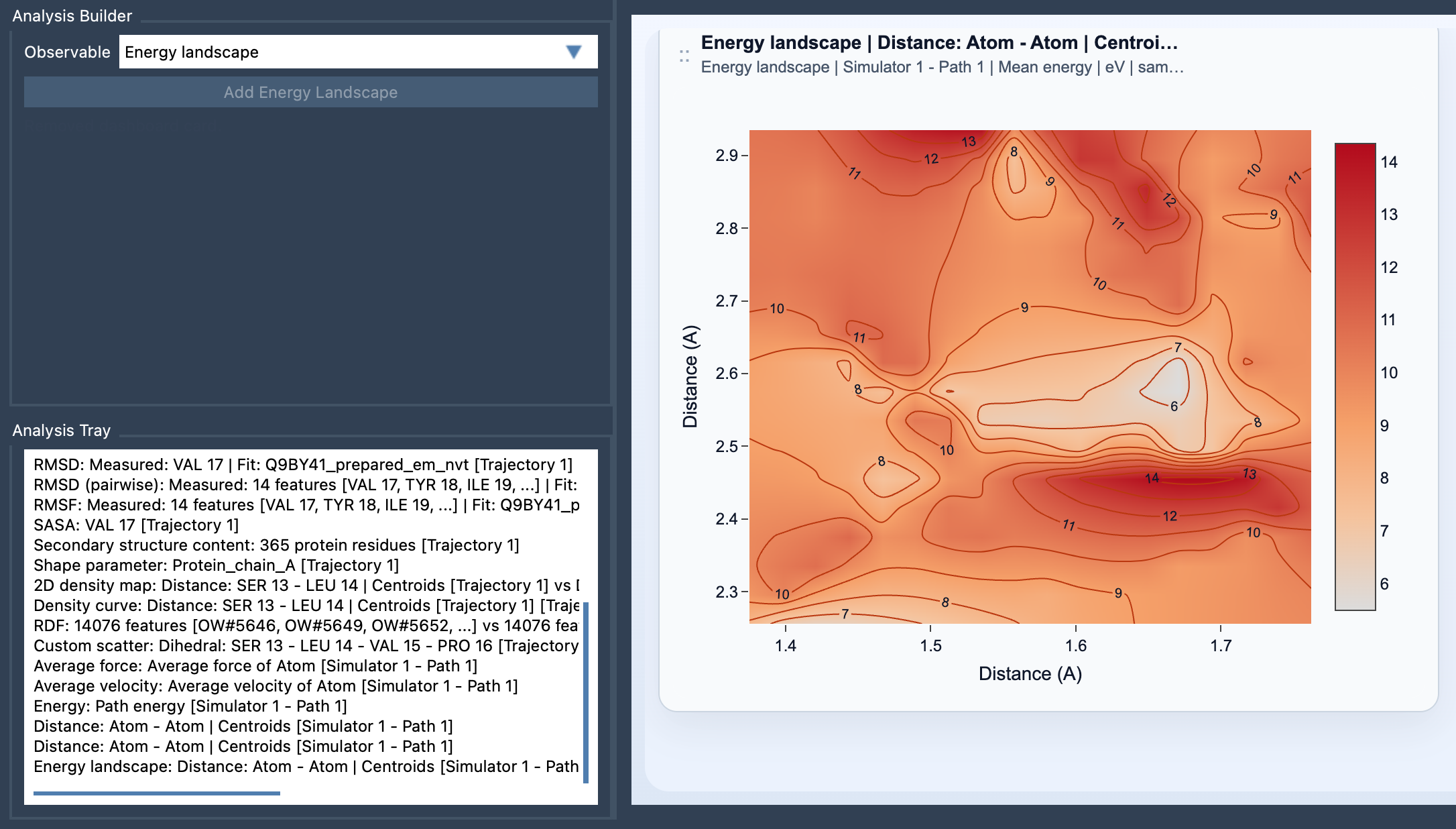
A molecular path can contain many frames, and inspecting them one by one makes it difficult to answer a practical question: where along this motion are the energetically interesting regions? A coordinate or distance plot may show how the structure changes, but it does not directly show how the path’s energy is distributed across those changes. The Energy Landscape view in SAMSON’s Path Analyzer brings those pieces together by projecting path energy onto two observables you choose.
Turn a long path into a map
Think of the two saved scalar analyses as the horizontal and vertical coordinates of a map. They might describe quantities such as a distance and RMSD, provided both analyses are frame-wise scalars calculated on the same path. Each path frame has values for those two observables and an energy value. Frames whose observable values fall into the same map cell contribute to that cell’s energy summary.
This is useful when a path is difficult to interpret from a sequence of structures alone. Instead of asking only what happens in each frame, you can look for regions of observable space associated with lower or higher sampled energies. Contours can make patterns easier to follow, while changing the color scale or energy unit can help make the display easier to inspect.
Mean or minimum: two different questions
For each cell, Path Analyzer can display either the Mean energy or the Minimum energy. The mean is the average energy of the frames that land in that cell. It gives a summary of the energies sampled there. The minimum is the lowest sampled energy among those frames; it highlights the most favorable energy value actually present in that bin.
These summaries answer different questions. Use the mean when you want to understand the typical energy of the sampled frames in a region. Use the minimum when you want to see the lowest sampled value reached there. A minimum should not be mistaken for the average behavior, and a mean can conceal an especially low-energy frame. Switching between the two is a straightforward way to see whether your interpretation depends on the summary statistic.
Build the view from compatible analyses
- Open Path Analyzer.
- Create or reuse two saved scalar analyses in the Analysis Tray.
- Choose Energy landscape as the observable and select exactly two saved scalar analyses.
- Click Add Energy Landscape.
Before creating the card, check that both source analyses are frame-wise scalar analyses computed on the same path, and that the path exposes energy data for the frames being considered. This view is derived from the Analysis Tray rather than from direct atom selections.
Read energy alongside sampling
An energy landscape summarizes energy in the space of two chosen observables; it is not the same as a map of how often the path visits each region. That distinction matters: a region can be interesting because of its energy, because it is frequently sampled, or because the path passes through it during a transition. If you want to separate energy trends from raw sampling density, compare the result with a 2D density map or Custom scatter.
A practical starting point is to choose two observables that distinguish the motion clearly—for example, Distance and RMSD—and then inspect both mean and minimum energy. Look for basins, possible transition regions, and routes connecting states, while keeping in mind that the view reflects the frames and energy data available on the path.
For the full setup and settings, see the Energy Landscape documentation.
Note: SAMSON and all SAMSON Extensions are free for non-commercial use. Get SAMSON.