



A molecular structure can look reassuringly familiar at a glance while parts of its backbone quietly change state along a path. The challenge is that viewing every frame—or inspecting residues one by one—can make it difficult to see the overall pattern. Is alpha structure becoming less prevalent? Is beta structure changing? Or is the selected region mostly staying in the same balance?
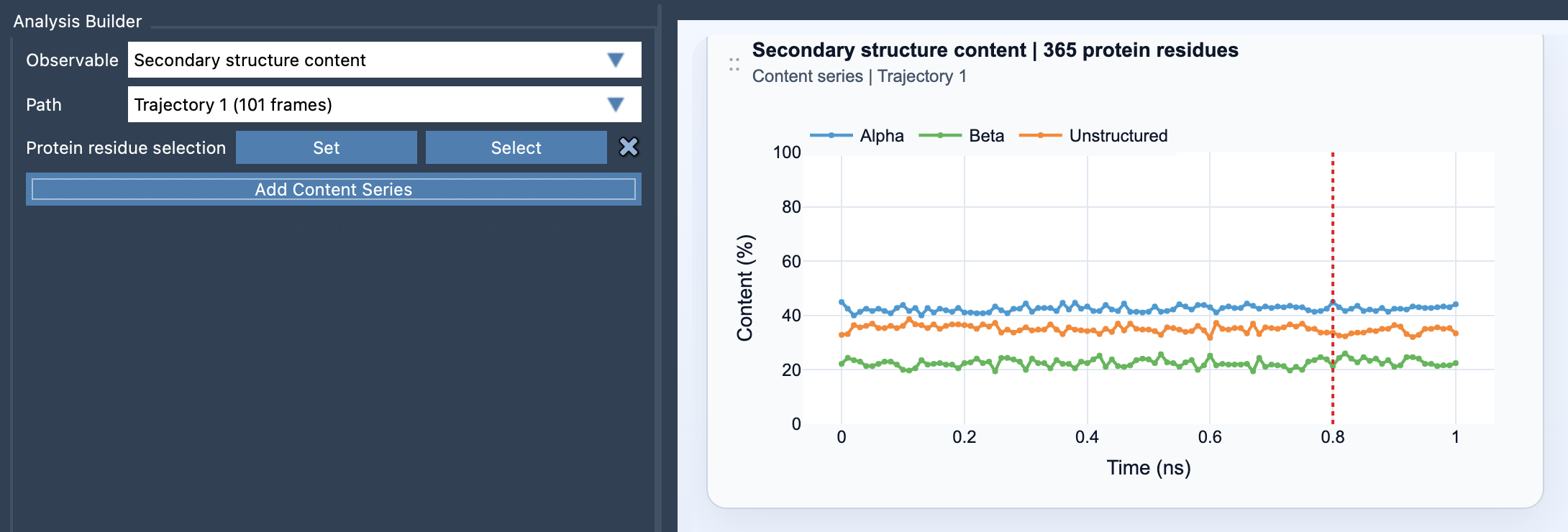
The Secondary structure content analysis in SAMSON’s Path Analyzer offers a compact way to answer those questions. It tracks the percentage of selected protein residues classified as Alpha, Beta, or Unstructured at each frame, then presents the values as a multi-series plot. That makes it useful as a first-pass summary of backbone-state changes across a path.
Start with the question you want to answer
Before adding a plot, decide whether you want a protein-wide overview or a closer look at one region. A broad residue selection can help you spot large-scale changes in the protein’s secondary-structure composition. A focused selection can help you follow a particular domain, helix bundle, or loop-rich region without the rest of the protein dominating the summary.
This choice matters: the percentages are calculated relative to the total number of selected protein residues. If you change the selection, you change the population being summarized. For a meaningful comparison between regions or analyses, keep track of exactly which residues are included.
What the plot measures
At each frame, Path Analyzer reports the percentage for each category. In simple terms, it divides the number of residues in that category by the total number of selected residues and multiplies by 100:
- Alpha: alpha-classified residue count divided by the selected residue count.
- Beta: beta-classified residue count divided by the selected residue count.
- Unstructured: unstructured residue count divided by the selected residue count.
Each plotted value therefore ranges from 0 to 100%. Read the lines as a changing composition of the selected region—not as a residue-by-residue map. For example, a declining Alpha percentage indicates that a smaller share of the selected residues is classified as alpha at that frame. The summary alone does not identify which residues changed or explain why.
Read trends, then investigate details
Look for sustained trends and changes that coincide with parts of the path you want to understand. A rise in one category alongside a decline in another can point to a shift in the region’s overall backbone-state composition. A relatively stable plot, by contrast, suggests that the proportions remain similar across the frames—even if individual residues may still differ.
One important interpretation check: a path’s frames represent progression along that path. Unless the path specifically corresponds to a time-resolved simulation trajectory, do not treat the horizontal axis as physical time or infer a rate of change from it. The plot summarizes states frame by frame; it does not, by itself, establish a mechanism or timescale.
Because the analysis aggregates residues, use it to find where to look next. If a region-level percentage changes, inspect the structure around the relevant frames to locate the residues involved. The Ramachandran analysis can complement this overview with residue-level backbone detail, helping connect a broad compositional trend to individual residues.
Add the analysis in Path Analyzer
- Open Path Analyzer.
- Choose Secondary structure content under Observable.
- Select a Path.
- Define a Protein residue selection. The selection must contain atoms belonging to protein residues.
- Click Add Content Series.
In short, this plot is most useful as a screening and comparison tool: it turns a changing structure into three easy-to-follow percentages, while leaving residue-level interpretation to follow-up inspection. For the complete instructions and equations, see the Secondary Structure Content documentation.
Note: SAMSON and all SAMSON Extensions are free for non-commercial use. Get SAMSON.