



A molecular structure can look crowded without telling you which contacts are common, and a list of pairwise distances can be difficult to interpret across a whole trajectory. The radial distribution function (RDF) offers a compact way to examine how the separation between two selected groups is distributed along a path. It can help investigate questions such as where solvent tends to sit around a solute, or which distances are characteristic of a ligand–pocket pair.
The key is to read the curve as a distance-dependent summary—not as a direct picture of a single structure. An RDF asks, in effect: how often do pairs from Group A and Group B occur at each separation? The result is a one-dimensional curve of density versus distance. Peaks can help identify distances where pairs are frequently found; the details depend on the selections, path, bin width, and whether the curve could be normalized.
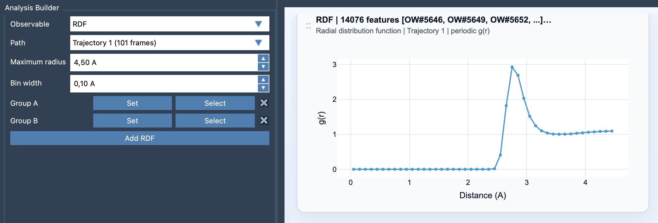
Set up a useful comparison
In SAMSON’s Path Analyzer, choose RDF as the observable, select a path, and define two atom-containing groups. Then set the maximum radius and bin width, and click Add RDF. The groups should reflect the question you want to answer: for example, a solute and its surrounding solvent, a ligand and a pocket selection, or two residue subsets.
Selection quality matters. If Group A or Group B includes atoms unrelated to the interaction you care about, the resulting curve combines those pairs too. A focused, chemically meaningful selection makes the analysis easier to interpret. Also remember that the two groups are required inputs; the plot summarizes distances between their atoms rather than displaying an individual contact.
Why the shell size matters
A raw distance count can be misleading. The volume of a thin spherical shell grows with distance: for radius r and shell thickness Δr, its volume is approximately 4πr2Δr. Consequently, more pairs may fall into shells farther from the center simply because those shells occupy more volume. In simplified terms, the count in a shell is related to the density at that distance multiplied by the shell volume.
This is why normalization is important when available. If valid periodic unit-cell information is present, Path Analyzer can normalize against the expected ideal-gas occupancy and report a properly scaled g(r). If periodic normalization is not possible, the app instead shows an RDF-style curve in arbitrary units. Treat that version as a relative, unnormalized summary: do not assume its values have the same scale or interpretation as a normalized g(r).
Choose resolution with the question in mind
The maximum radius sets how far out the distribution is sampled. Choose a range that covers the distances relevant to your comparison; a very large range may add little if you are investigating only nearby packing. Bin width controls radial resolution. Narrow bins can reveal finer features, but can also make a curve noisy; wider bins smooth the picture but may blur nearby features. There is no universally best setting, so use a resolution suited to the distance scale and the amount of sampled data.
Finally, interpret the RDF in context. A peak marks a distance range with a stronger population in the plotted distribution; it does not, by itself, establish why the groups are there or prove a particular chemical interaction. Pair the curve with your structural understanding and the selections used to produce it. And because RDF cards summarize the path globally, they are not linked to a single frame: the plot describes the path as a whole, not one moment in it.
For the setup details and notes on inputs, normalization, and interpretation, see the RDF documentation.
Note: SAMSON and all SAMSON Extensions are free for non-commercial use. Get SAMSON.