



A common challenge in molecular modeling is turning two known protein structures into a useful transition path. The endpoints may show the same protein in different conformations, yet differ in residue count or structural coverage. A direct interpolation can then be awkward: the structures do not correspond perfectly, and the resulting path may need refinement before it is useful to inspect.
The SARS-CoV-2 spike opening example offers a concrete way to think through that problem. It uses the closed spike structure, PDB 6VXX, and the open structure, PDB 6VYB. The goal is not to claim that a computed path is an experimentally observed movie. Rather, the workflow creates an illustrative route between known endpoint conformations and makes the assumptions and limitations visible.
First, understand what the motion represents
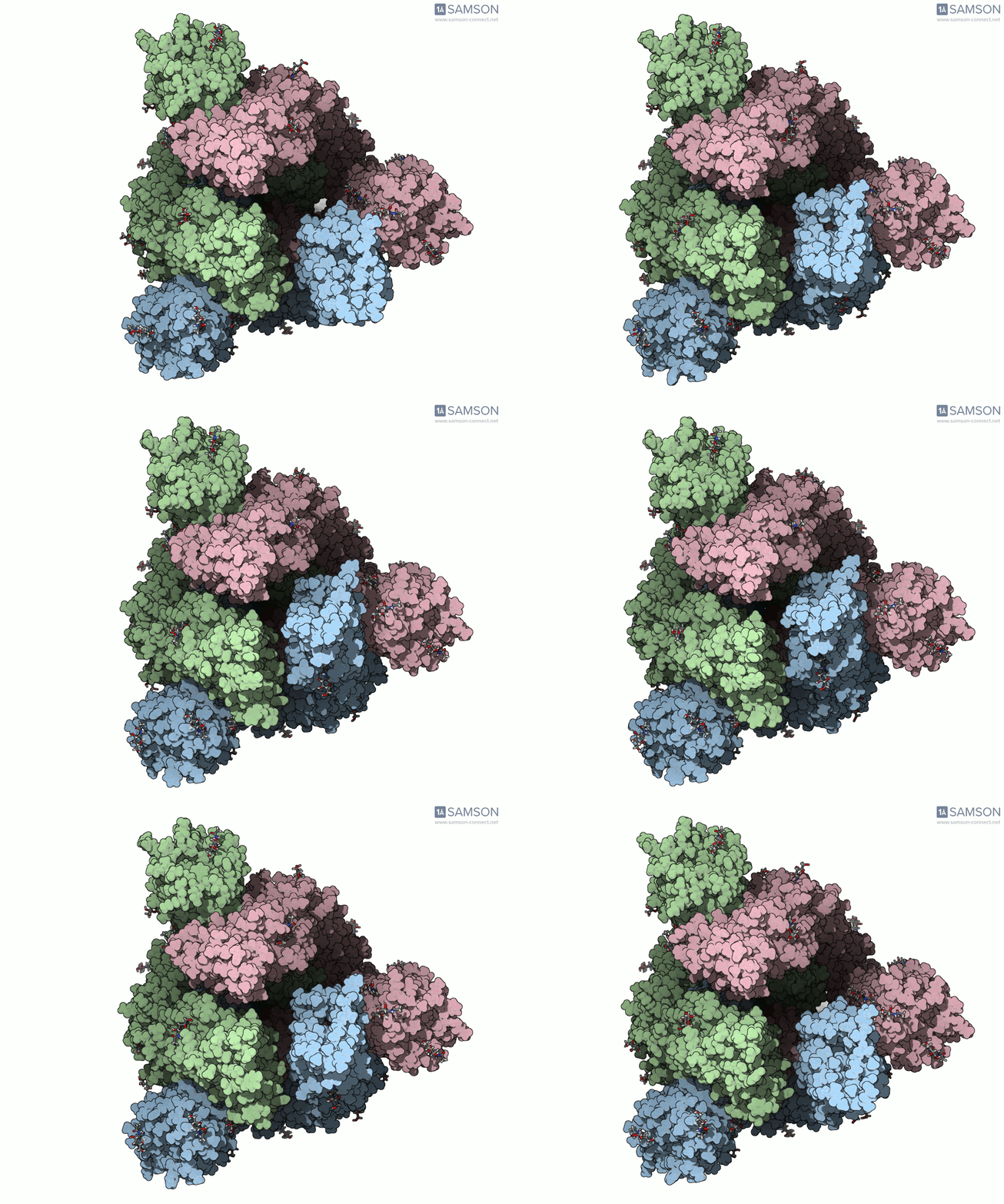
The spike is a three-protein assembly. In its closed, or down, state, the receptor-binding region is less exposed; in an open, or up, state, it can engage ACE2 on a host cell. Seeing the protein move between these states helps explain why a static structure alone can be an incomplete picture of a molecular process.
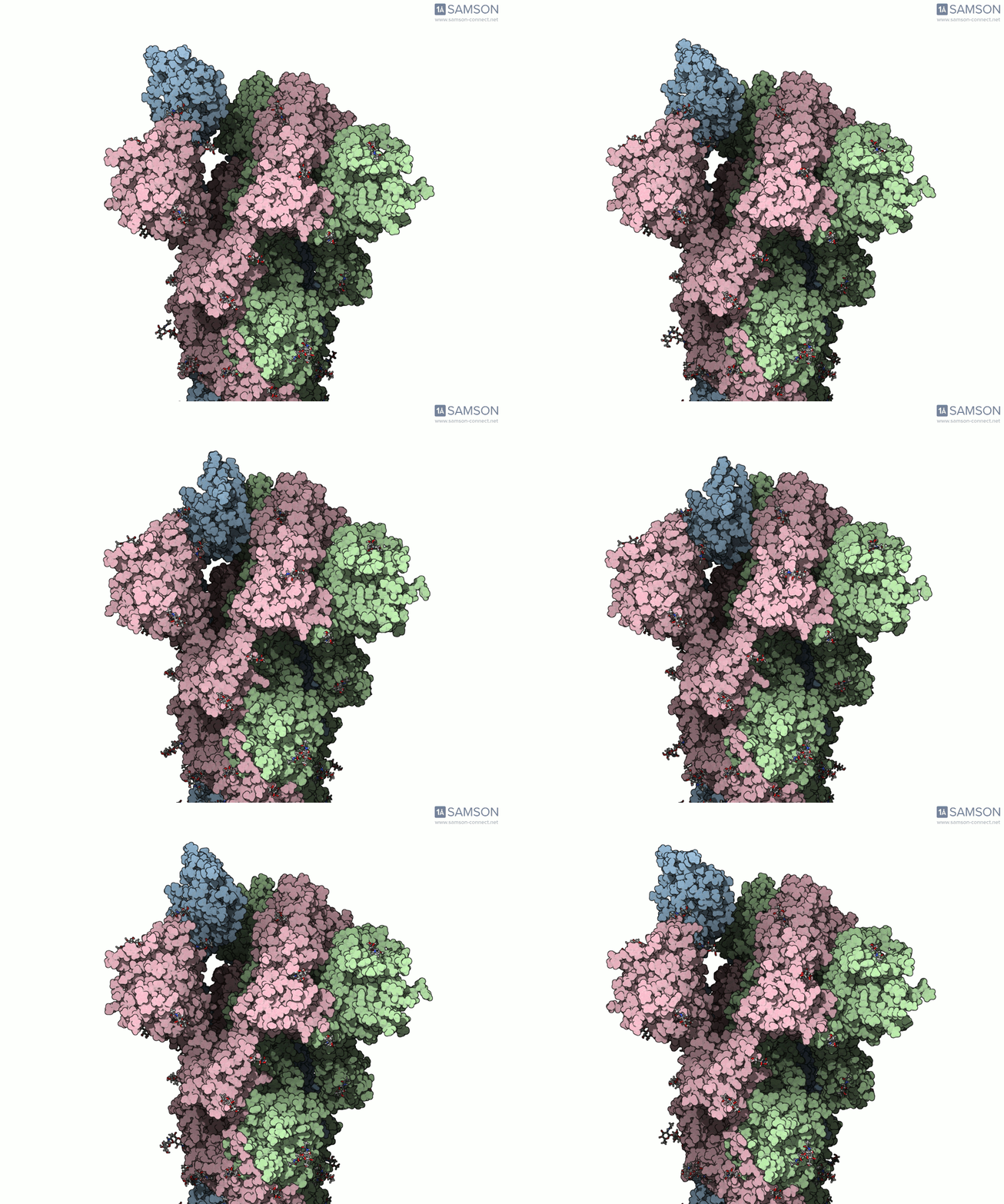
The animation is useful for orientation, but it should not be mistaken for a measured timescale or a validated biological trajectory. A computed path is a model-derived sequence of conformations connecting structures, not proof that the protein follows that exact route in cells.
A workflow that handles mismatched endpoints
The example begins with preparation. Bond orders in the sugar molecules are adjusted, because this is needed before adding hydrogens. Hydrogens are then added to both structures, followed by minimization. This preparation matters: a path calculation depends on the structures it receives, so basic chemical setup should be addressed before interpreting the motion.
Next, the ARAP Interpolation Path module generates an initial path between the endpoint structures. In the documented setup, the open structure (6VYB) is used as the starting conformation and the closed structure (6VXX) as the goal. A key complication is that the endpoint structures contain different numbers of residues. The initial path corresponds to the starting structure, so the workflow uses a conformation along that path to construct a compatible closed-state conformation, then minimizes it.
This is a useful general lesson: when two structures are not directly compatible, do not treat interpolation as a black box. Check which atoms or residues the generated path actually represents, and make sure the endpoint used for refinement has the same structural basis as the path. Matching the representations is part of the modeling problem, not a cosmetic detail.
With the prepared closed-state conformation available, the interpolation is generated again. The P-NEB (Parallel Nudged Elastic Band) module is then used to improve the path. In this example, the initial ARAP path took less than half a minute on a laptop, while the P-NEB refinement took about 15 minutes. Those timings are specific to the reported workflow and hardware, but they illustrate the distinction between quickly generating a first path and spending additional computation to refine it.
Inspect, then validate
The example trajectory is available as individual PDB files, a single PDB trajectory, or a SAMSON file. The SAMSON file includes the spike structure, open and closed conformations, and paths from ARAP and P-NEB; the conformations and animation can be explored in the document view. These formats make it easier to inspect the path and choose a workflow that fits your analysis.
Keep the caveat close at hand: the supplied trajectories are provided as is and have not been experimentally verified. They may be useful for visualization or further calculations, but may require post-processing and validation for a particular research question. A smooth-looking animation is not, on its own, evidence that every intermediate structure is physically realistic.
For the full walkthrough, downloadable files, and details of the modules used, see the original spike-opening documentation.
Note: SAMSON and all SAMSON Extensions are free for non-commercial use. Get SAMSON at samson-connect.net.