



A molecular trajectory can produce many useful measurements: distances, energies, RMSD, radius of gyration, solvent-accessible surface area, and more. The challenge is that separate plots make it hard to see how two measurements change together. Does a distance increase as energy changes? Do conformations with larger RMSD also have a larger radius of gyration? A custom scatter plot puts two saved scalar analyses into one view, making these relationships easier to examine.
From two curves to one comparison
Imagine that you have calculated a distance and an energy along a molecular path. Looking at each analysis separately can tell you how each value changes over the sampled frames, but it may not immediately show whether particular distance values tend to occur alongside particular energy values. A scatter plot pairs the two scalar values for each sample: one value is plotted against the other, and each point represents one sampled pair.
This changes the question from “How does each measurement vary?” to “Which values occur together?” Depending on the shape and distribution of the points, you may notice an apparent relationship, an opposing trend, distinct groups, or a region worth investigating as a possible transition. These are observations to explore—not proof that one measurement causes the other.
Build the comparison in Path Analyzer
- Open Path Analyzer.
- Create or reuse two scalar analyses and make sure they are saved in the Analysis Tray.
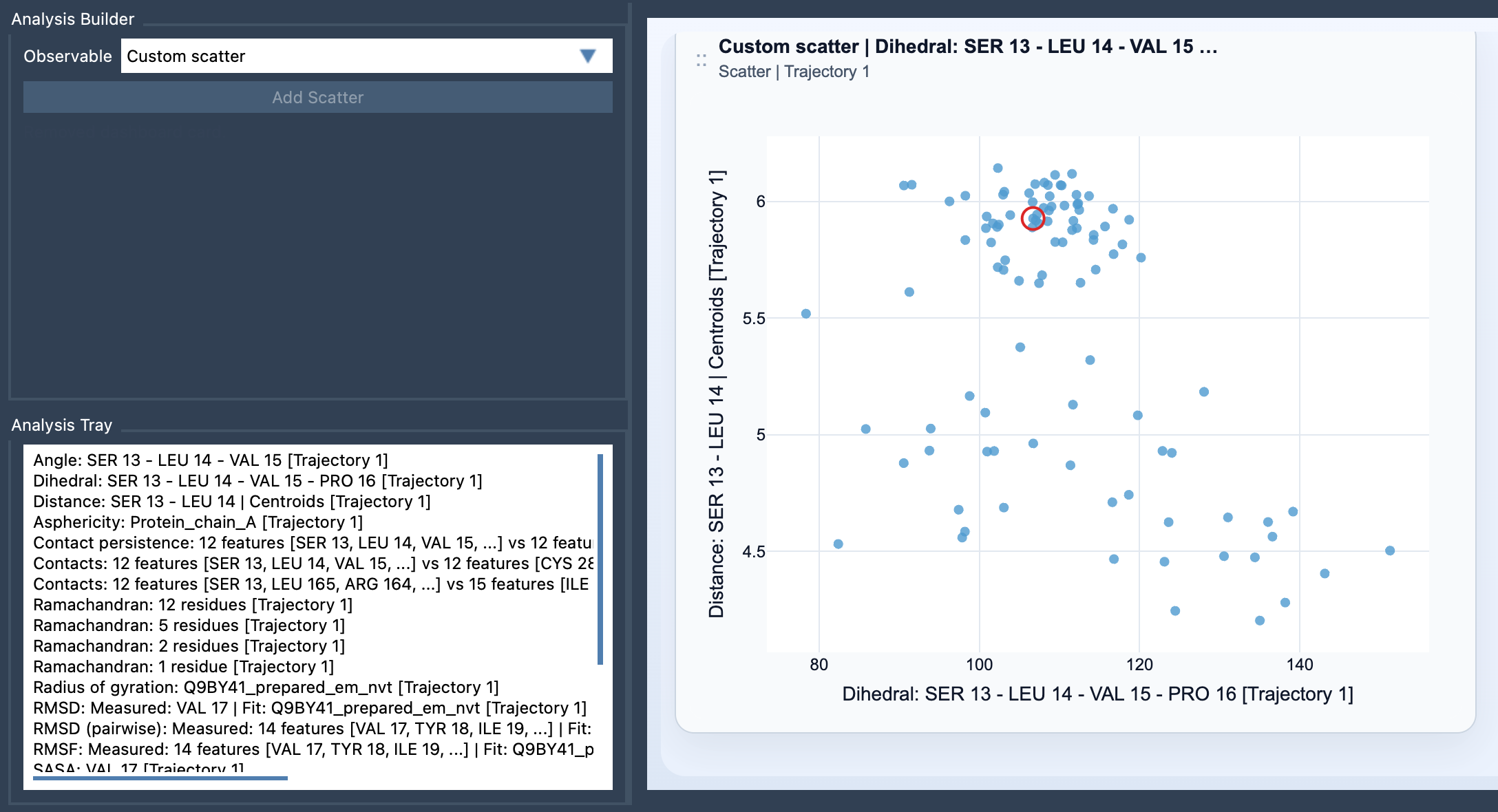
- Choose Custom scatter under Observable.
- Select exactly two saved scalar analyses in the tray, then click Add Scatter.
Custom scatter is a derived analysis, so its inputs come from the Analysis Tray rather than from direct atom selections. Both source analyses must be scalar analyses. Before adding the plot, it helps to name the scientific question you want it to address: for example, “How does distance vary with energy?” or “Do larger-RMSD samples also show a larger radius of gyration?” A focused pair is usually easier to interpret than a comparison chosen simply because two analyses happen to be available.
Read the points in context
Start by looking at the overall arrangement. Are the points spread broadly, concentrated in a small region, or separated into visible groups? Is there a pattern that would be obscured if you considered each measurement only on its own? Treat these as prompts for closer inspection. A scatter plot compares the sampled values; by itself, it does not explain why a pattern occurs or establish a causal mechanism.
When both source analyses come from the same path and remain frame-linked, the scatter plot can stay connected to the current frame. In this case, clicking a point can move the path to its corresponding frame. That interaction is useful when a point catches your attention: you can relate the paired measurements back to the molecular structure at that position in the path, rather than treating the plot as an isolated summary.
Use the scatter as a first step
A custom scatter plot can help you decide what to investigate next. For instance, if the distribution suggests that the relationship changes across different regions, you may want a view that makes those regions easier to examine. The documentation points to a 2D density map and an Energy landscape as possible next visualizations. The scatter plot is a practical starting point: first compare two observables, then choose a follow-up view that fits the question raised by the data.
For the exact setup steps and input requirements, see the Custom Scatter documentation.
Note: SAMSON and all SAMSON Extensions are free for non-commercial use. Get SAMSON.