



A protein structure can look convincing in 3D and still contain backbone conformations worth checking. That matters when you are preparing a model for refinement, simulation, or molecular design: strained or unusual residues may be easy to miss when inspecting the structure one residue at a time.
A Ramachandran plot offers a compact way to inspect this part of a protein. It maps each residue’s backbone dihedral angles, φ (phi) and ψ (psi), against one another. Regions of the plot indicate conformations that are energetically favored or unfavorable. The plot does not replace broader structure validation, but it can help you spot where a closer look may be useful.
Start with a structure-wide view
In SAMSON, open the Interactive Ramachandran Plot from Home > Apps > Biology > Ramachandran plot, then click Update to generate the plot for the current protein. In the example below, yellow areas represent energetically favorable regions, while white areas represent unfavorable conformations.
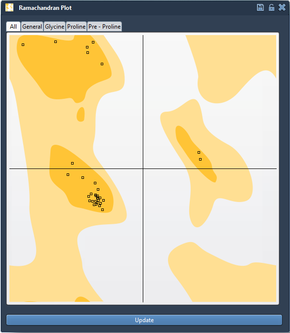
This view helps turn a broad question—“Are there backbone conformations I should investigate?”—into a more focused one: “Which residues are outside or near the favored regions?” Use the category tabs to inspect all residues together or filter the plot to General, Glycine, Proline, or Pre-proline residues. These categories make it easier to interpret residues in context rather than treating every amino acid as though it had identical conformational preferences.
Connect a plot point to the 3D structure
A point is not just a mark on a chart. Click one to select its residue in the molecular viewport, and check the status bar for its φ and ψ values. This makes it possible to move between the overview and the structure: identify a point that deserves attention, select the corresponding residue, and inspect where it sits in the protein.
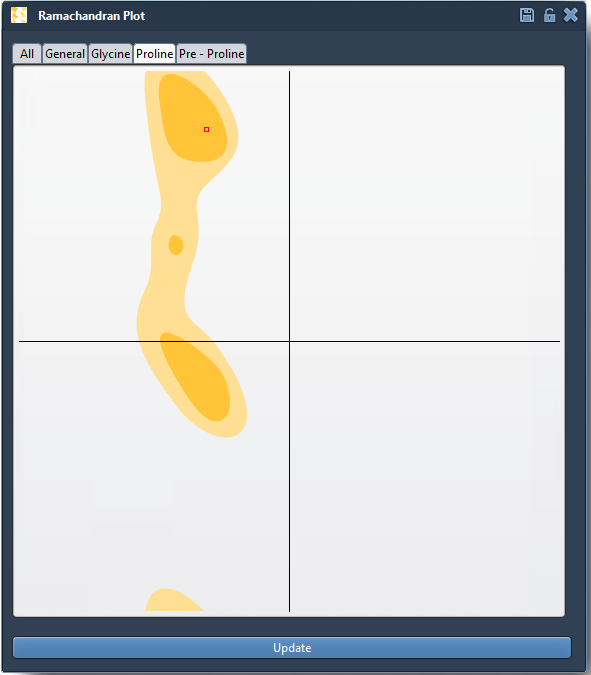
That connection is useful when an unusual conformation appears. Instead of relying on the plot alone, you can locate the residue in 3D and decide whether it is relevant to the modeling task. The plot highlights conformational information; interpretation still depends on the structure and the question you are trying to answer.
Make local changes, then reassess
If a conformation needs adjustment, there are two interactive approaches described in the tutorial. Drag a point in the plot to change its dihedral angles and see the 3D structure update. Or select the Twister editor in the viewport and twist the protein in 3D while watching the plot update. If a plot edit does not produce a result you want, use Ctrl+Z on Windows or Linux, or Cmd+Z on macOS, to undo it.
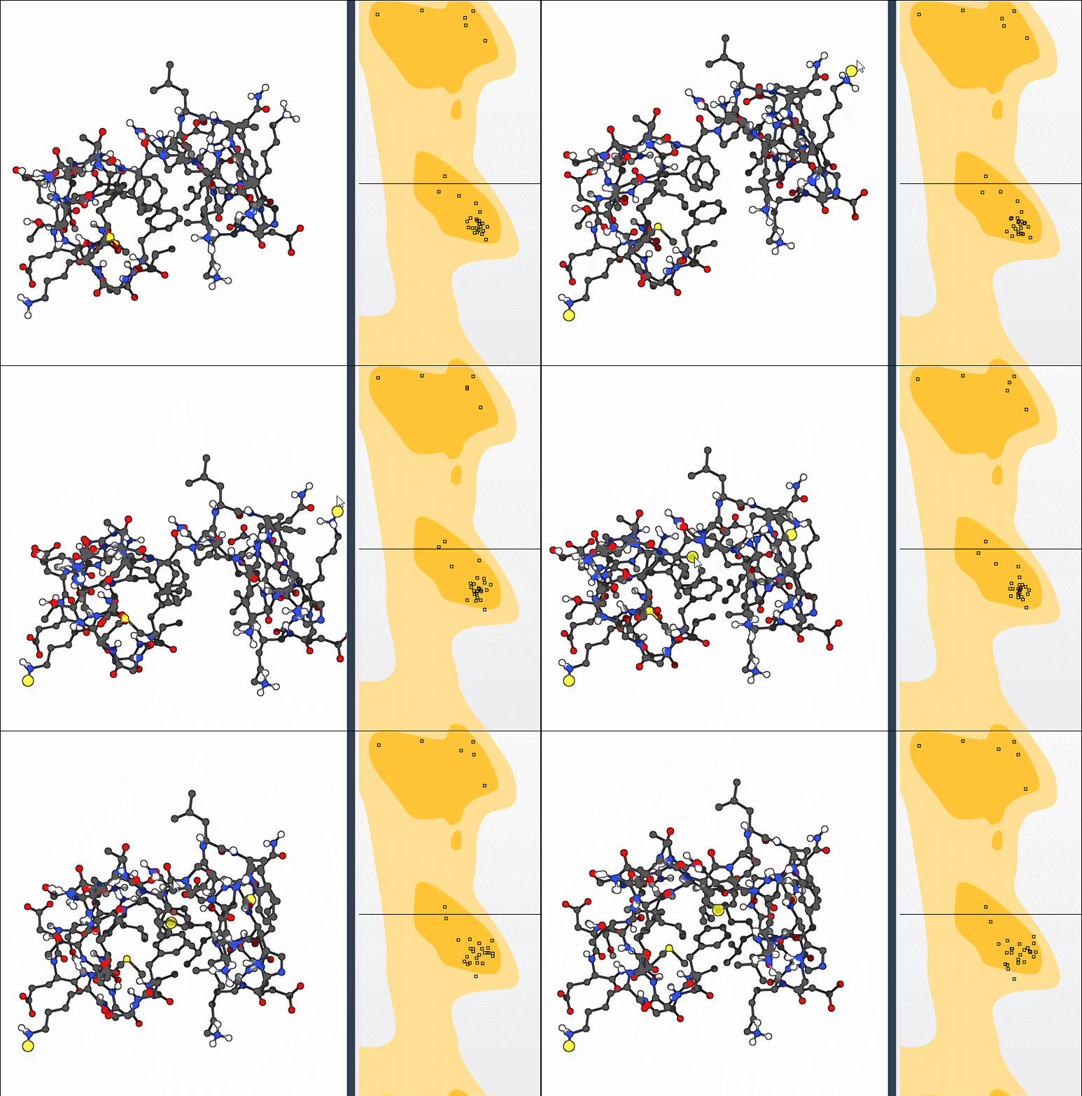
A practical way to use these controls is to make a deliberate change, then check both views again: the residue’s position in the plot and its placement in the 3D structure. Avoid treating movement into a favored region as an automatic guarantee that the whole model is correct. The plot is one useful lens for examining backbone conformations, not a substitute for other preparation and validation steps.
Use it as part of a modeling workflow
For a quick exercise, load the example protein with PDB ID 1YRF, update the plot, and inspect the residue categories. You can also explore the tutorial’s bonus challenge: compute the first 10 nonlinear normal modes, shift the first mode fully left with a scaling factor of 1, then use the Ramachandran plot to adjust conformations toward favored regions. This combines a global motion with local inspection, while keeping the backbone-angle view available as you work.
Whether you are checking a homology model, investigating a binding-site residue, or preparing a structure before simulation, the key benefit is the feedback loop: identify a residue, connect it to the 3D model, make a considered edit if needed, and inspect the result again.
For setup details and the full workflow, see the Interactive Ramachandran Plot tutorial.
Note: SAMSON and all SAMSON Extensions are free for non-commercial use. Get SAMSON.